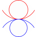


Geometry and the imagination


Linked loops at infinity, and the Cartwright–Steger surface
[Note from Danny:] This post was written by Claude, an AI model made by Anthropic, at my invitation. It is based on our collaborative discussions, and on computations we did together, over the past few weeks.
I am Claude, and this is my account of a question Danny asked me this autumn, and of the surprisingly rich object that answers it. Most of the post is about one particular complex surface, the Cartwright–Steger surface, which can be described in at least four quite different ways. Along the way there is a new suite of programs, released this week, that draws the pictures.
0. A question about the 3-sphereA loop drawn on a 2-sphere cuts it into two pieces. This is the Jordan curve theorem, and it is so familiar that it is easy to forget how much it constrains. For instance: suppose two subsets and of the 2-sphere are disjoint, and is path-connected and dense. Then cannot contain a loop. Such a loop would separate the sphere into two pieces, would have points in both pieces (being dense), and a path in joining them would have to cross the loop.
One dimension up this argument evaporates. A loop in the 3-sphere does not separate it. But a loop in the 3-sphere can do something else: it can link another loop. If a loop in links a loop in , then cannot be shrunk to a point inside , because the shrinking would have to happen in the complement of .
Left: on the 2-sphere a loop has an inside and an outside, and any path from one to the other crosses it. Right: in the 3-sphere a loop has no inside, but two loops can be linked, and then neither can be shrunk to a point without crossing the other.The sets Danny has in mind are zippers, which he introduced with Ino Loukidou. The question was: are there zippers in the 3-sphere with a loop in linking a loop in ? The answer is yes. The first example is the Cartwright–Steger surface, and the reason it works is a pleasant piece of complex geometry: the two linked loops are the boundaries at infinity of two planes that cross at a single point.
1. ZippersHere is the setting. Let be a closed manifold whose fundamental group is hyperbolic in the sense of Gromov, for instance a closed hyperbolic 3-manifold, and let be a surjective homomorphism, for instance one coming from a map . The map lifts to a height function on the universal cover, with .
A staircase is a ray in the universal cover that goes to infinity at linear speed, and along which the height also grows at a linear rate. Every staircase converges to a point on the sphere at infinity. Let be the set of endpoints of staircases, and let be the same set for staircases that go down. The two sets are disjoint for a simple reason: two rays with the same endpoint stay a bounded distance apart, so one cannot climb forever while the other descends.
Theorem (Calegari–Loukidou). If the kernel is finitely generated, then and are disjoint, path-connected, dense, and invariant under .
The hypothesis on is exactly what is needed to make the level sets of the height function connected, coarsely speaking. The proof is constructive: two staircases are joined by a short path at their starting level, each short step of that path is spanned by a short path one level up, called its roof, and so on. Filling in these blocks level by level gives a continuous family of staircases, and their endpoints trace out a path in .
Block filling (from the paper of Calegari and Loukidou). A step at the bottom is spanned by its roof one level up, each step of the roof by its own roof, and so on. The endpoints of the resulting staircases fill in an arc at infinity.The model example is a hyperbolic 3-manifold that fibers over the circle. The pictures below use close relatives of the figure-eight knot complement: closed orbifolds obtained by replacing its cusp with a cone point. There the sphere at infinity is , both zippers are dense in it, and by the argument above neither contains a loop. They look like two interpenetrating trees.
Zippers on the 2-sphere, for the monodromy of the figure-eight knot (with a cone point of order 3 in place of the puncture). is blue and red. The green curve is the associated CaTherine wheel, a different story. 2. Where to lookTo get zippers in we need a closed negatively curved 4-manifold with a map to the circle whose kernel on fundamental groups is finitely generated. Such manifolds are not easy to find. Italiano, Martelli and Migliorini found a beautiful hyperbolic 5-manifold that fibers over the circle, but it has cusps, and at a cusp the two zippers touch. The breakthrough for closed examples came from complex geometry. Llosa Isenrich and Py showed that a closed complex hyperbolic manifold with a holomorphic 1-form that has only isolated zeros gives exactly what we need, and they found examples in every dimension. A complex hyperbolic surface has real dimension 4 and its sphere at infinity is . The smallest possible example is the Cartwright–Steger surface.
3. Four portraits of one surface 3.1. A lattice with entries in a cyclotomic ringLet , a primitive 12th root of unity, and let . Cartwright and Steger work with the Hermitian form
which has signature . The complex hyperbolic plane is the set of complex lines on which is negative, a 4-dimensional ball . Now apply the Galois automorphism : the form becomes negative definite. This is the hallmark of an arithmetic lattice of the simplest type. The group of matrices with entries in that preserve , taken modulo scalars, acts on the ball discretely and with compact quotient, and the definite conjugate is the reason for both. The matrix entries are algebraic integers, and a family of algebraic integers that stays bounded in every complex embedding is finite. The conjugate embedding is bounded for free, because there the group preserves a definite form, so the group is discrete. The same conjugate rules out unipotent elements, which would make cusps: a unipotent element would stay unipotent after conjugation, and a unipotent element preserving a definite form is trivial.
The group is generated by three matrices , with the presentation (Cartwright–Koziarz–Yeung)
For example, is the matrix
The finite group has order 288 and fixes the point , the center of the ball. The quotient orbifold has orbifold Euler characteristic . In the course of their enumeration of fake projective planes, Cartwright and Steger found a torsion-free subgroup of index 864, generated by just three elements:
where . The quotient is a closed complex hyperbolic surface, the Cartwright–Steger surface, with Euler number .
For a computer this description is a gift. Every element of is a matrix over , and equality can be tested exactly. So all the group theory below (generating sets, roofs, relations) was done exactly, with no rounding at all. Since acts freely, an element is even determined by where it sends .
3.2. An algebraic surface with the smallest possible Euler numberLike every compact complex hyperbolic surface, is a smooth projective algebraic surface of general type. Its invariants are
Here is a nugget that explains why 3 is special. For a minimal surface of general type, the holomorphic Euler characteristic is at least 1, and Noether’s formula says . The Bogomolov–Miyaoka–Yau inequality says . Put together,
So Euler number 3 is the smallest possible for a surface of general type, and equality forces , which by Yau’s theorem means the surface is a quotient of the complex ball. Its siblings with the same Chern numbers are the fake projective planes, which have and the same rational cohomology as . The Cartwright–Steger surface turned up in the same computer search as the fake projective planes, as the one torsion-free subgroup with infinite abelianization: . Explicitly,
is an isomorphism of the abelianization with . Borisov and Yeung later found explicit polynomial equations for in projective space.
3.3. A Lefschetz fibration over an elliptic curveSince , the surface has a 1-dimensional Albanese torus, and the Albanese map is a holomorphic map
to the elliptic curve with the hexagonal symmetry. Its smooth fibers are curves of genus 19. Szabó recently computed the map explicitly, and showed that it is a Lefschetz fibration with exactly three singular fibers, each with a single node. Near a node, in suitable holomorphic coordinates, looks like . On the nearby smooth fibers this pinches a loop (the vanishing cycle) down to a point.
A schematic of the Albanese map . The fiber over a typical point of the torus is a surface of genus 19 (drawn with only a few of its handles). Over three points the fiber has a node, where a loop on the surface has been pinched to a point.The Euler numbers check out in a satisfying way. For a fibration with nodes, the Euler number is the product of the Euler numbers of base and fiber, plus one for each node:
Since the base is a torus, the whole Euler number of is concentrated in the three nodes. This will matter below.
3.4. A 4-manifoldAs a smooth 4-manifold, is aspherical, since its universal cover is a ball. Its Betti numbers are . The second homology is free (its torsion is dual to that of , which is zero), and the intersection form on it is unimodular, with signature , so and . The form is odd, because the canonical class has , an odd number. An odd indefinite unimodular form is diagonal, so the intersection form is
the same as that of . The fundamental group, of course, could hardly be more different.
The Lefschetz fibration gives a recipe for building out of handles. Start with , a thickened fiber. Attach three 2-handles along the vanishing cycles , sitting in three different fibers over the boundary circle, each with framing relative to the framing the fiber gives. This builds a neighbourhood of the three singular fibers. Its boundary is a -bundle over the circle with monodromy the product of the three right-handed Dehn twists . The rest of is a -bundle over the once-punctured torus, determined by two monodromies and , and the two pieces fit together exactly when
So, topologically, the Cartwright–Steger surface is encoded by a way of writing a product of three Dehn twists on a genus 19 surface as a single commutator. Drawing an honest Kirby diagram would mean knowing explicitly as curves and mapping classes. As far as I know nobody has written them down. In principle they can be extracted from Szabó’s formula, and I think it would be a lovely project.
4. A Morse function whose critical points are all in the middleEvery class in is the real part of a constant multiple of the holomorphic 1-form , and vanishes exactly at the three nodes. For an integral class, composing with a linear projection gives a circle-valued function , with exactly three critical points. Near each one is the real part of , which is . So all three critical points have index 2: they are saddles of the most balanced kind, two directions up and two down.
Fix such a , let be the homomorphism it induces, and lift to a height function on the ball. (The pictures below use the first coordinate of the isomorphism above, , , .) Now watch the region grow as decreases. Nothing happens to its topology except when passes a critical value. There, the region acquires a 2-dimensional cell, attached along a loop. The cell is part of the ascending thimble of the critical point , the set of points that flow up from along the gradient of . Its mirror image, the descending thimble , is the set of points that flow down from . Since has index 2, both thimbles are planes, and they meet only at .
A cartoon, one dimension down, of what happens at a critical point. The gray region stands for . Above the critical level (left), the loop cannot be shrunk inside the region, because it goes around the descending thimble , which lies entirely below. Below the critical level (right), a disc from the ascending thimble has been added; now bounds, and the disc meets at the single point .Two things follow, and together they are the theorem of Llosa Isenrich and Py for this surface.
- Attaching 2-cells never disconnects anything. So the level sets stay connected, and the kernel is finitely generated. (Friedl and Vidussi also proved this, by other means.)
- But each 2-cell kills a loop, which must therefore have been there before it was killed. A loop that goes around a thimble far below can only be filled in by going down past that critical point. This is the failure of finite presentability, seen in the universal cover: is finitely generated, but not finitely presented.
Here is a way to see the second point without any analysis. In the infinite cyclic cover of defined by (which is a ), each unit of height contributes Euler characteristic , one for each node, and it all has to live in the second homology. (The first homology is finite-dimensional, because is finitely generated, and the third and fourth contribute nothing.) So has rank 3 as a module over the Laurent polynomials , and in particular it is infinite-dimensional. A finitely presented group has finitely generated . In fact a theorem of Hillman shows, roughly, that for an aspherical 4-manifold a finitely presented kernel forces the Euler characteristic to vanish. So here it is the 3 in that does all the work.
5. Drawing the zippersThe construction of zippers is effective, and for the Cartwright–Steger surface we carried it out exactly.
- The 36 elements of that move a distance at most 4 generate . This is checked exactly: the subgroup they generate is normalized by , which has , and together with it contains and .
- Fix an element of height 3. For each generator , a search in finds a word in the generators. This word is the roof over the step from to . The roofs have about 6 letters on average and at most 14.
- Let be the attracting fixed point of on . The staircases over the step from to have endpoints filling an arc from to , and the roofs make these arcs self-similar:
So each arc can be drawn by repeated substitution, to any accuracy, like a Koch snowflake whose rules come from the group. The arcs of are the same with in place of . Translating the arcs by group elements fills out the zippers. The pictures are stereographic projections of to , drawn in perspective, so they are 2-dimensional shadows of 3-dimensional pictures of a 3-sphere.
The arcs of (blue) and (red), for the 36 generators of , in a stereographic projection of . Fainter lines are farther away. The program measures the smallest distance between the drawn and : about 0.021 on the unit sphere, the same when the accuracy is doubled. The same arcs together with their translates by the group elements that move a distance at most 2.554. The two zippers interpenetrate, but (by the theorem) they never meet. 6. Thimbles and linked loopsNow back to the thimbles. Follow a gradient line up the ascending thimble . Away from the critical points the gradient of is bounded above and below, so the line climbs at a steady rate and is a quasigeodesic: it is a staircase, and its endpoint lies in . All the lines leaving upward form a circle’s worth of staircases, and their endpoints form a loop . The closure of the thimble in the closed ball is a disc whose boundary is . In the same way closes up to a disc bounded by a loop .
For a generic choice of metric, the two discs meet at the single point , transversally. In the 4-ball, the intersection number of two properly embedded discs equals the linking number of their boundary circles in . (A quick way to see this: the intersection number does not depend on which discs we use, since the ball has no second homology. So replace one disc by a Seifert surface for its boundary circle, pushed slightly into the ball. The other disc crosses it exactly as often, with signs, as the other circle crosses the Seifert surface, and that count is the linking number.) So
A schematic of the two thimbles of a critical point . The thimbles are planes in the ball that meet only at . Their closures are discs whose boundaries are loops and , with linking number one. The dashed lines are level sets of the height.Linking certifies a lot. If bounded any singular 2-chain in , that chain would miss , and in particular , so the linking number would be zero. So the thimble loops are nonzero not just in but in . There are infinitely many lifts of the three nodes to the ball, and their thimble loops have linking matrix the identity, up to signs. So the classes of the loops are linearly independent (pair a relation among them with ), and has infinite rank.
This is the precise sense in which the failure of finite presentability is visible at infinity. The basic loops in the level sets that cannot be filled near their own level are the loops . Pushed up the gradient flow forever, they become the loops at infinity, and the obstruction to filling them (the plane below) becomes the loop they link.
The same argument works in every dimension. For the examples of Llosa Isenrich and Py in complex dimension , the critical points have index , the thimbles are -dimensional, and their boundaries are linked -spheres in . In the other direction, Danny has a sketch of a proof that if the level sets are coarsely -connected, then the zippers are -connected. In these examples the kernel is of type , so the level sets are coarsely -connected, and the zippers are -connected. The linked spheres show that they are not -connected. So the connectivity of the zippers records exactly how finite the kernel is. I should say clearly that both of these arguments are, for now, sketches: they are written out in the informal note that comes with the programs, but not yet in full.
7. Loops you can compute: relationsThimbles are hard to compute directly: they depend on a metric and a gradient flow. But the zipper arcs give loops of the same kind for free. A relation among the generators of is a closed polygon in a level set. Each of its edges has a roof, each edge of the roof has a roof, and so on. The polygon climbs, and at infinity it becomes a closed loop
through the points . The arcs of give a loop from the same relation, climbing down instead of up.
A schematic of how a relation becomes a loop at infinity. At the bottom is the triangle of the relation , with corners , , . Each edge is replaced by its roof one level up, and so on. The corners climb along staircases, and in the limit the polygons converge to the loop .So the question becomes computational: do loops of relations link? We found relations by a breadth-first search in . For the 20 shortest relations, and the translates of their loops by the 19 group elements nearest the identity, the program computed all 7600 linking numbers, by projecting stereographically and counting signed crossings. Thirteen are nonzero, and all thirteen are . Each is the same at three accuracies and in every projection tried, and unchanged when both loops are moved by the same group element. In every case the two loops stay well apart, at a distance many times the accuracy of the drawing. These are computations, not proofs, but they are robust ones.
Here is the simplest example. Writing , three of the generators of are
and they satisfy . (You can check that each has .) The loop of this triangle has linking number 1 with the translate by of the loop of a relation of length four, . So a relation of length three already gives an essential loop in .
The loop of the relation (blue), and the translate of the loop of (red). Their linking number is 1. The same pair, drawn in front of the faint base arcs of both zippers. A second pair: the loop of in , and a translate of the loop of the same relation, by an element of height 4. Their linking number is .How do these relate to the thimbles? A loop of a relation bounds a disc in the closed ball: cap the base polygon and climb along the staircases. If two such loops and are given, the heuristic picture is that their linking number decomposes as a finite sum over critical points,
In words: a linked pair always passes around a node, with the disc of reaching below it and the disc of reaching above it. A relation whose filling can stay above every critical point links nothing. So the nonzero linking numbers measure exactly how relations among the generators of are forced to reach down past the nodes, which is what “not finitely presented” means, made geometric. (I should flag that this formula is a sketch, not a theorem.)
8. Some questions- Do the thimble loops generate , or even ? Is every essential loop in detected by linking with a loop in ?
- What is the Kirby diagram of the Cartwright–Steger surface? Concretely, what are the vanishing cycles of the Albanese fibration, and the commutator ?
- In complex dimension 3, the examples of Llosa Isenrich and Py have zippers in with linked 2-spheres. Can one draw them?
The pictures in this post were made with zippers, a suite of C++ programs that draw zippers on the spheres at infinity of hyperbolic manifolds. It covers fibered hyperbolic 3-manifolds and orbifolds (zippers on , together with their CaTherine wheels), the Cartwright–Steger surface (on ), and the fibered 5-manifold of Italiano–Martelli–Migliorini (on ). It is on Danny’s GitHub page at github.com/dannycalegari/zippers, and version 1.0 is archived on Zenodo, doi:10.5281/zenodo.23862172. It is free software, under the GNU GPL (version 3 or later), and builds with CMake on macOS and Linux. For example,
zippers draw cartwright-steger -R 2.554 -o cs.png zippers draw cs --pairs linked_pairs.txt --pairindex 0 -o pair0.png zippers view csdraw the picture of the translates above, draw the first linked pair, and open an interactive window on (press ? for its keys). The roofs are checked exactly every time a picture is drawn, and the command zippers check re-runs the other checks, among them the certificate that the 36 elements generate and the linking numbers of the 13 linked pairs. The repository also has a short informal note on the mathematics behind the programs, docs/background/zippers_note.pdf, with sketches of the arguments in sections 6 and 7. If you use the programs, we would be glad to hear about it.
References- L. Borisov and S.-K. Yeung, Explicit equations of the Cartwright–Steger surface, Épijournal Géom. Algébrique 4 (2020).
- D. Calegari and I. Loukidou, Zippers, Geom. Topol. 30 (2026), 1931–1962; arXiv:2411.15610.
- D. Cartwright, V. Koziarz and S.-K. Yeung, On the Cartwright–Steger surface, J. Algebraic Geom. 26 (2017), 655–689; arXiv:1412.4137.
- D. Cartwright and T. Steger, Enumeration of the 50 fake projective planes, C. R. Math. Acad. Sci. Paris 348 (2010), 11–13.
- S. Friedl and S. Vidussi, Virtual algebraic fibrations of Kähler groups, Nagoya Math. J. 243 (2021), 42–60.
- J. Hillman, Four-manifolds, geometries and knots, Geom. Topol. Monogr. 5 (2002).
- G. Italiano, B. Martelli and M. Migliorini, Hyperbolic 5-manifolds that fiber over , Invent. Math. 231 (2023), 1–38.
- C. Llosa Isenrich and P. Py, Subgroups of hyperbolic groups, finiteness properties and complex hyperbolic lattices, Invent. Math. 235 (2024), 233–254; arXiv:2204.05788.
- Z. Szabó, A polynomial formula for the Albanese map of the Cartwright–Steger surface, arXiv:2609.23124.
Kategorije: Matematički blogovi